


Graphs are everywhere. From modeling molecular interactions and social networks to detecting financial fraud, learning from graph data is powerful—but inherently challenging.
While Graph Neural Networks (GNNs) have opened up new possibilities by capturing local neighborhood patterns, they face limitations in handling complex, long-range relationships across the graph. Enter Graph Transformers, a new class of models designed to elegantly overcome these limitations through powerful self-attention mechanisms. Graph Transformers enable each node to directly attend to information from anywhere in the graph, capturing richer relationships and subtle patterns.
In this article, we’ll introduce Graph Transformers, explore how they differ from and complement GNNs, and highlight why we believe this approach will soon become indispensable for data scientists and ML engineers alike.
Where are Graph Transformers making an impact?
Here are just a few examples of where they’re already proving powerful:
- Protein folding and drug discovery
- Fraud detection in financial transaction graphs
- Social network recommendations
- Knowledge graph reasoning and search
- Relational Deep Learning
What are Transformers?
Imagine analyzing data where relationships between elements matter more than their individual values. Transformers address this challenge through their attention mechanism, which automatically weighs the importance of connections between all elements in your dataset. This allows the model to focus on what's relevant for each prediction, creating a flexible architecture that adapts to the data rather than forcing data to fit a rigid structure.
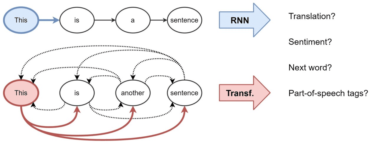
What distinguishes Transformers architecturally is their parallel processing capability. Unlike recurrent models that process sequences step-by-step, Transformers compute self-attention across all positions simultaneously. This parallelization not only accelerates computation but enables the model to capture long-range dependencies without the vanishing gradient problems that plague sequential models. By combining this with positional encodings and multi-head attention, Transformers achieve state-of-the-art performance across diverse domains while maintaining computational efficiency.
More formally: Given a set of tokens, each token is associated with a feature vector . The self-attention mechanism in Transformers computes new representations for each token by aggregating information from all other tokens in the set. For each token , the self-attention mechanism involves the following steps:
1. Linear Projections
The first step in self-attention is to transform the input token representations into three different spaces: Query , Key , and Value . These are obtained by applying learned linear transformations to the original input features
where represents the feature vectors of all tokens, and are trainable weight matrices. The Query represents the "search criteria" each token uses to find relevant information, the Key acts as an "identifier" to determine how relevant a token is to others, and the Value holds the actual information to be aggregated. The goal is to allow the model to selectively attend to relevant parts of the input while ignoring irrelevant ones.
2. Scaled Dot-Product Attention
Once we have the Query and Key matrices, we compute the attention scores between every pair of tokens using the dot product of their queries and keys:
This formula determines how much attention each token should pay to every other token. The softmax function normalizes these scores so that they sum to 1, ensuring a proper probability distribution. The scaling factor prevents the dot product values from becoming too large, which can lead to very small gradients during training. Finally, these attention weights are applied to the Value matrix, meaning that each token aggregates information from all others based on their computed relevance. This mechanism allows the model to capture long-range dependencies and relationships across the entire input.
3. Multi-Head Attention
Instead of computing a single attention score for each token pair, multi-head attention improves the model’s expressiveness by running multiple attention mechanisms in parallel. Each attention head learns different aspects of the relationships between tokens
where each attention head is computed as
Each head has its own set of projection matrices , allowing it to focus on different types of relationships (e.g., syntactic vs. semantic in NLP or local vs. global patterns in graphs). The outputs of all attention heads are then concatenated and linearly projected using to combine the diverse learned information. Multi-head attention allows the model to capture a richer set of interactions and prevents it from focusing too narrowly on any single aspect of the data.
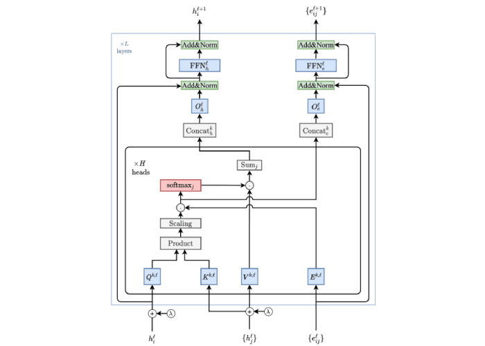
4. Feedforward and Residual Connections
After multi-head attention, the output is passed through a position-wise feedforward network (FFN) that applies additional transformations to improve expressiveness. This step consists of two fully connected layers with a non-linearity in between, typically a ReLU or GELU activation function. To ensure stability and ease of training, residual connections and layer normalization are used:
The residual connections help mitigate the vanishing gradient problem, allowing deeper networks to be trained effectively. Layer normalization ensures that activations remain well-conditioned, improving convergence and generalization. This final step refines the learned representations, ensuring that they effectively capture the complex relationships necessary for the task at hand.
Together, these steps allow Transformers to model intricate dependencies across all tokens in an input sequence, making them highly effective for tasks that require understanding global and contextual relationships.
What is a Graph Transformer?
A Graph Transformer adapts the core attention mechanism of traditional Transformers to work on graph-structured data. Instead of processing sequences, it attends over nodes and edges — capturing both local structure and global context without relying on step-by-step message passing like GNNs.
By integrating relational and structural information directly into the attention layers, Graph Transformers can model arbitrary graph topologies, long-range dependencies, and heterogeneous relationships — all while retaining the scalability and parallelism that make Transformers so powerful.
In the next sections, we’ll break down how Graph Transformers compare to traditional Transformers and GNNs, and what makes them especially suited for complex relational data.
Comparing Transformer and Graph Transformer
While traditional Transformers revolutionized sequence modeling, Graph Transformers adapt this architecture to handle the complex relational structure of graphs. The key distinction lies in how Graph Transformers incorporate graph topology directly into their attention mechanisms, allowing them to model node relationships regardless of sequential position.
Graph Connectivity
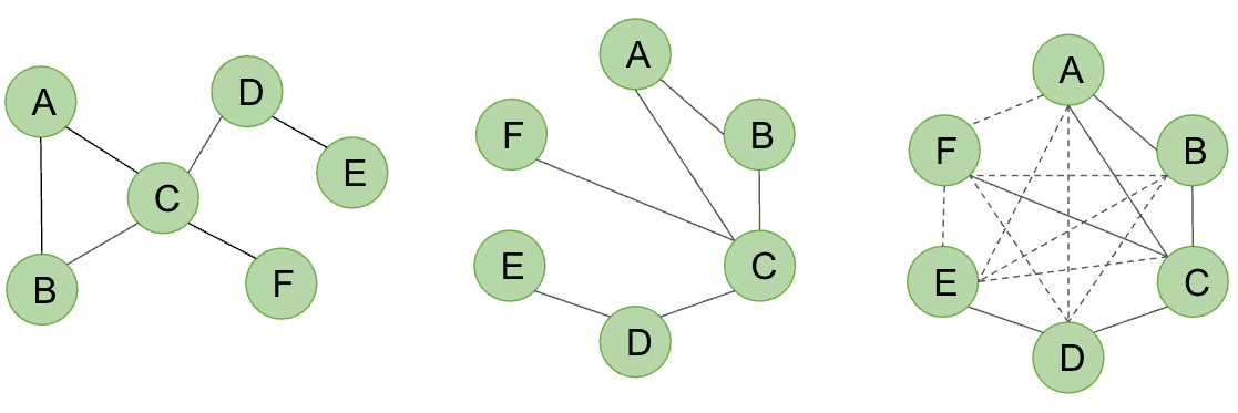
A traditional Transformer treats its input as a fully connected graph, where every token (or node) can directly attend to every other token. While this global attention mechanism is powerful, it does not leverage any inherent structural information present in real-world graphs. Additionally, when dealing with large datasets containing millions or billions of nodes, maintaining full connectivity quickly becomes computationally infeasible.
On the other hand, a Graph Transformer introduces an inductive bias by incorporating the graph’s topology into the attention mechanism. Instead of allowing every node to attend to all others, nodes primarily focus on their local neighbors, similar to GNNs. This localized attention reduces computational costs while ensuring that the model respects the graph structure. By balancing global attention with local connectivity, Graph Transformers efficiently capture both long-range dependencies and fine-grained relational patterns, making them well-suited for large-scale graph datasets.
Positional Encodings
In standard Transformers used in language models, positional encoding is crucial because words in a sentence are processed in parallel, meaning their order must be explicitly encoded. Since words in different positions can have different meanings, Transformers incorporate positional encodings to provide a sense of sequence. This allows the model to distinguish between phrases like "dog bites man" and "man bites dog", even though they contain the same words. These encodings are absolute and follow a well-defined order, ensuring that the Transformer understands the linear structure of text.
In Graph Transformers, however, there is no predefined order of nodes like in a sentence. Instead, positional encodings serve a different purpose: capturing the structural relationships between nodes within the graph. Rather than encoding a sequential position, Graph Transformers encode where a node is located relative to others, helping the model understand proximity, hierarchy, and connectivity. Since graphs vary widely in structure—ranging from simple social networks to complex molecular structures—designing effective positional encodings is a challenging and active area of research. In fact, this topic is so fundamental to improving Graph Transformers that we dedicate an entire section later in this blog to exploring different strategies for Graph Positional Encoding in depth.
Edge Awareness
In standard Transformers, the attention mechanism operates over a fully connected set of tokens, where each token can directly attend to every other token. There are no inherent node features because natural language sequences, images, and many other data types typically lack explicit relationships between individual elements beyond their positions. In NLP, for example, the interaction between words is implicitly learned through self-attention weights rather than being explicitly defined as an edge with associated features.
However, in Graph Transformers, edges often carry crucial information that defines the relationships between nodes. In domains like molecular graphs, edges represent chemical bonds with different types and strengths; in social networks, edges may encode the type or frequency of interactions between users. Ignoring edge information would mean losing important structural context. To address this, Graph Transformers incorporate edge features directly into the attention mechanism, but different architectures handle this in different ways. Some approaches modify the attention score by integrating edge attributes into the key-query similarity computation, while others introduce edge-aware message-passing mechanisms or additional embeddings that explicitly encode edge properties. The ability to incorporate edge information makes Graph Transformers significantly more expressive than their standard counterparts when applied to relational data.
We summarize the main differences between standard transformers and Graph Transformers in the following table:
| Aspect | Standard Transformer | Graph Transformer |
|---|---|---|
| Data Structure | Ordered sequences | Graphs |
| Attention Scope | Fully connected (all tokens) | Can be local (based on graph structure) |
| Positional Encoding | Absolute (sinusoidal, learned) | Graph-aware |
| Edge Awareness | No explicit edge modeling | Explicitly incorporates node and edge features |
| Computational Complexity | O(N²) | Reduced via neighborhood constraints |
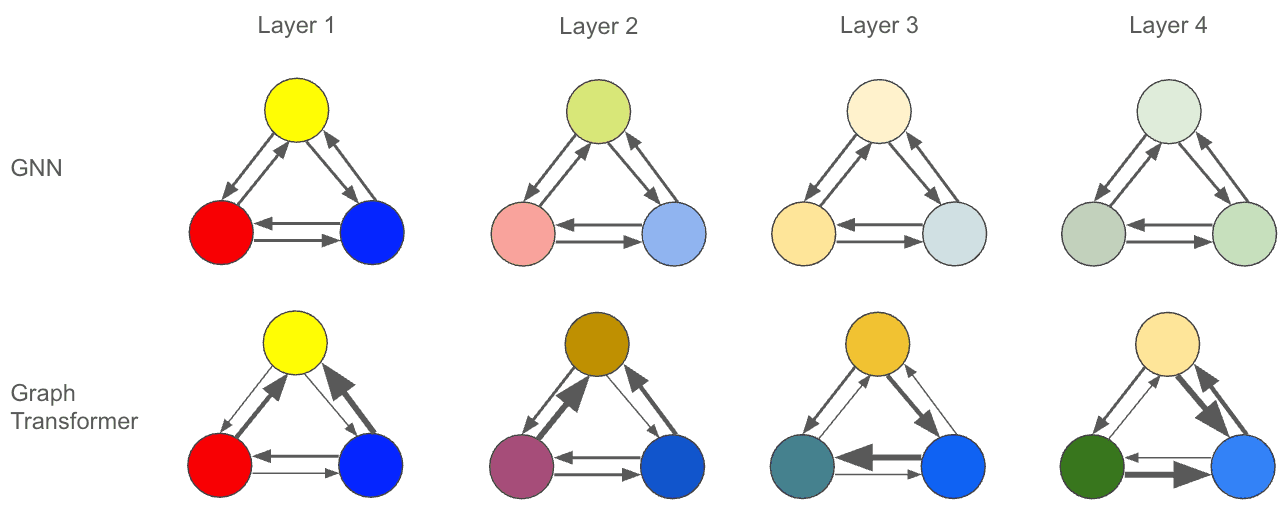
Comparing GNN and Graph Transformer
Graph Neural Networks (GNNs) have revolutionized graph representation learning, primarily through message passing neural networks (MPNNs). These models excel at capturing local structural information by iteratively aggregating and transforming feature vectors from neighboring nodes. This sequential message passing approach defines a node's representation based on its immediate connectivity, limiting the scope of information flow to local neighborhoods. While effective, this approach introduces several challenges, especially as graphs grow larger and more complex.
Graph Transformers, inspired by the success of Transformers in natural language processing, offer an alternative paradigm. Instead of relying on this localized message passing, they treat the graph as a fully-connected structure and leverage self-attention mechanisms to capture global dependencies across the entire graph. This fundamentally different perspective aims to address several critical challenges encountered with traditional GNNs.
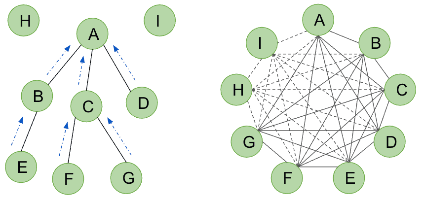
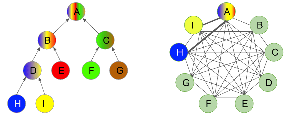
Information Flow
GNNs perform sequential message passing means that information propagates through the graph layer by layer, with each node's representation updated based on its direct neighbors. This process is inherently local, limiting the reach of information to nodes within a certain "hop" distance. Graph Transformers, on the other hand, consider the graph as fully-connected. In this case every node in the graph is considered as potentially connected to every other node (unless explicit restrictions are imposed). Self-attention mechanisms calculate attention weights that determine the importance of each node relative to all others, regardless of their distance. This allows for direct capture of global dependencies and enables a more nuanced and flexible representation of node relationships.
Long-range Dependencies
A key distinction between Message Passing Neural Networks (MPNNs) and Graph Transformers lies in their handling of long-range dependencies. MPNNs, relying on localized message passing, face challenges in efficiently capturing interactions between distant nodes; as network depth increases, information from far-off nodes becomes progressively diluted. In contrast, Graph Transformers, leveraging self-attention, enable any node to directly attend to any other node within the graph, irrespective of their separation. This ability to capture global dependencies is particularly vital in tasks like molecular property prediction, where interactions between distant atoms can significantly influence overall properties. This advantage is especially pronounced in small but sparse graphs, such as molecular graphs, where the graph diameter can be substantial relative to the number of nodes, making long-range dependencies crucial.
Over-Smoothing
A notable challenge encountered with deep Message Passing Neural Networks (MPNNs) is the phenomenon of over-smoothing. As the network depth increases, node features tend to converge towards similar values, resulting in a loss of discriminative information. This homogenization of node representations can hinder the model's ability to distinguish between different nodes and capture nuanced structural patterns. Graph Transformers, in contrast, are inherently less susceptible to over-smoothing. Their self-attention mechanism allows nodes to retain their individual characteristics, as each node can attend to all others with varying degrees of importance. This ability to preserve distinct features mitigates the tendency for features to become homogeneous, offering a significant advantage in tasks requiring fine-grained node differentiation.
Over-Squashing
Another critical limitation of MPNNs is the over-squashing problem. This issue arises from the aggregation of messages from numerous neighbors into a single node representation, creating an information bottleneck. As information is compressed through successive message passing layers, crucial structural details can be lost, restricting the model's ability to capture complex patterns. Graph Transformers, however, do not operate within the same message passing framework. By employing self-attention, they circumvent the need for such aggregation, thus avoiding the information loss associated with over-squashing. This architectural difference allows Graph Transformers to maintain a more comprehensive and detailed understanding of the graph's structure, enabling them to effectively model intricate relationships without the constraints imposed by information bottlenecks.
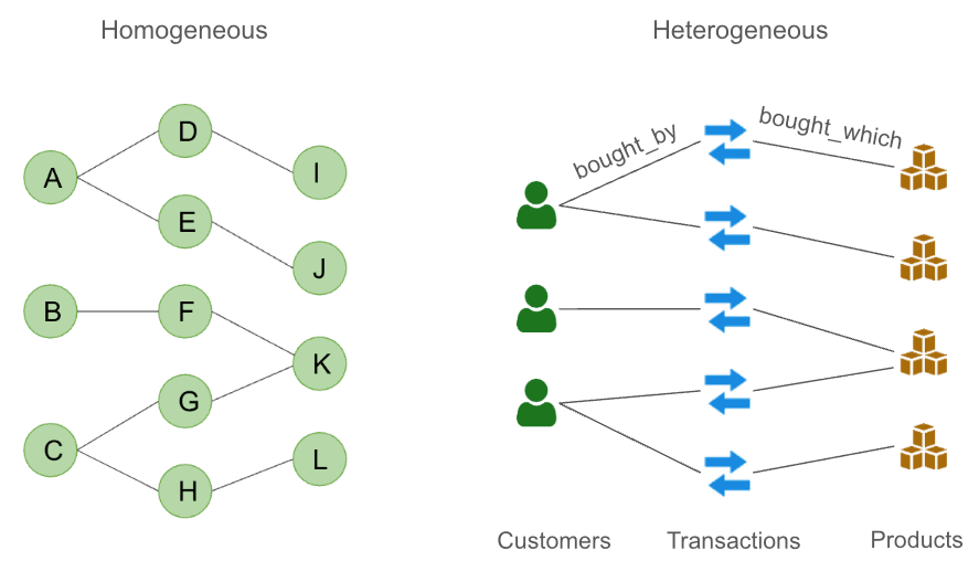
Heterogeneous vs. Homogeneous Data
While Transformers were originally designed for homogeneous sequential data, like text, their application to graph-structured data presents a unique challenge, as many real-world graphs exhibit heterogeneity. This heterogeneity can manifest in the form of diverse node and edge types, as well as varying relational semantics. Traditional Transformers, with their inherent assumption of uniform data, require adaptation to effectively handle such complex graph structures. Fortunately, similar to the evolution of GNNs towards handling heterogeneous graphs, Graph Transformers have also seen significant advancements in this area. Techniques like those presented in "Heterogeneous Graph Transformer" and related works have introduced mechanisms to incorporate type-specific information and relational biases into the self-attention process. These adaptations enable the model to distinguish between different node and edge types, and to learn type-aware representations that better capture the intricate relationships within heterogeneous graphs. This ongoing research demonstrates the adaptability of the Transformer architecture, extending its capabilities beyond homogeneous data and paving the way for more robust and versatile graph representation learning.
This table highlights how Graph Transformers address many of the core limitations of traditional GNNs while offering greater flexibility for modeling complex, heterogeneous graphs.
| Aspect | Graph Neural Networks | Graph Transformers |
|---|---|---|
| Information Flow | Sequential message passing between connected nodes. | Self-attention allows direct aggregation from all nodes. |
| Long-Range Dependencies | Struggle with distant relationships due to limited hops. | Capture long-range dependencies more effectively. |
| Over-Smoothing | Node embeddings become too similar with deep layers. | Less prone, as attention allows flexible information mixing. |
| Over-Squashing | Information gets compressed when aggregating many neighbors. | Mitigated by attention, distributing information more effectively. |
| Heterogeneous Models | RGCN, HAN, HGT | HGT, Graphormer, HEAT |
Positional and Structural Encoding
Understanding positional encodings is crucial for Graph Transformers to process relational data effectively. Since transformers naturally treat each subgraph as fully connected, where every node can directly interact with any other, positional information helps the model understand the structure of the data. Without it, the model would have no way of distinguishing between nodes based on their relative positions, leading to a loss of important relational context. Here we highlight main trends for positional and structural encoding employed with Graph Transformers.
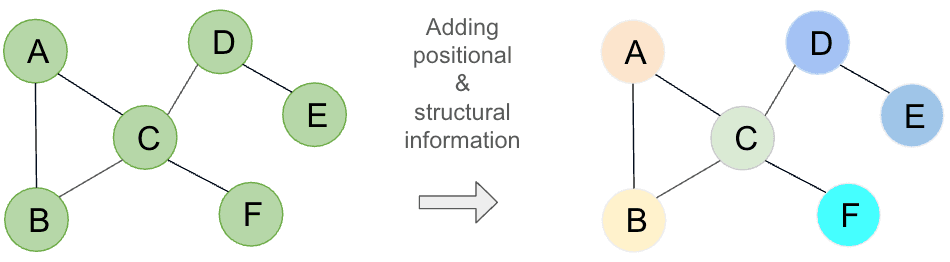
Positional Encoding
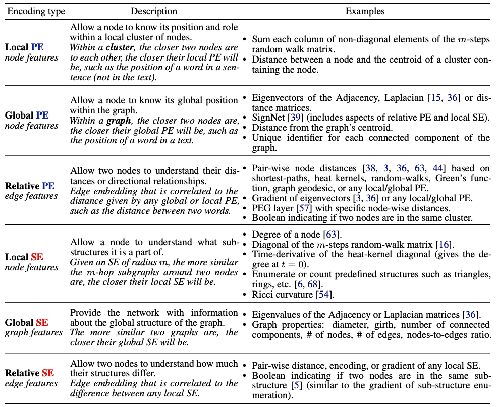
Positional Encodings provide nodes with a sense of their location within the graph, answering the question, "Where am I?". Given the topological nature of graphs, determining a node's position isn't straightforward. Therefore, the following methods can be employed:
- Local PEs (Node-Level): These encodings reflect a node's position relative to a specific substructure or cluster within the graph. Nodes that are closer within a cluster will have similar local PEs. Examples include, the distance between a node and the centroid of its cluster, or the sum of non-diagonal elements in the m-step random walk matrix, indicating the node's reachability within m steps.
- Global PEs (Node-Level): These encodings provide a node's position concerning the entire graph. Nodes that are closer in the overall graph structure will have similar global PEs. Examples include eigenvectors of the adjacency or Laplacian matrix, which capture the graph's spectral properties, the distance from the node to the graph's centroid, or assigning a unique identifier for each connected component, distinguishing nodes in different subgraphs.
- Relative PEs (Edge-Level): These encodings represent the positional relationship between pairs of nodes, often correlating with the distance between them. Examples include pairwise distances derived from heat kernels or random walks, indicating how information diffuses between nodes, or gradients of eigenvectors from the adjacency or Laplacian matrices, capturing changes in spectral properties between nodes.
Structural Encoding
Structural Encodings provide insights into the local and global architecture of the graph, helping to answer, "What does my neighborhood look like?". They can be categorized as follows:
- Local SEs (Node-Level): These encodings help a node understand the substructures it participates in. Nodes with similar local neighborhoods will have similar local SEs. Examples include node degree, diagonals of the m-step random walk matrix, or counting specific substructures like triangles or rings that the node is part of, providing insights into local connectivity patterns.
- Global SEs (Graph-Level): These encodings offer information about the overall structure of the graph. Graphs with similar global structures will have similar global SEs. Examples include eigenvalues of the adjacency or Laplacian matrices, summarizing the graph's spectral characteristics, or graph properties such as diameter (the longest shortest path between any two nodes), number of connected components, and average node degree.
- Relative SEs (Edge-Level): These encodings capture structural differences between pairs of nodes, highlighting how their local neighborhoods compare. Examples include gradients of local SEs, indicating changes in local structures between nodes, or boolean indicators denoting whether two nodes share the same substructure, such as being part of the same ring or clique.
Dealing with Large Graphs in Graph Transformers
Working with very large graphs poses significant computational challenges for Graph Transformers, primarily due to the quadratic complexity of the self-attention mechanism. Here we highlight a few techniques you can apply to make Graph Transformers feasible for large graphs.
Sparse Attention Mechanisms
These models modify the attention mechanism to attend only to a subset of nodes, reducing the computational cost. Techniques include:
- Local Attention: Attending only to neighboring nodes, similar in spirit to GNNs but with the flexibility of attention weights.
- Global Attention with Selected Nodes: Attending to a small set of global "anchor" nodes in addition to local neighbors. See “GOAT” and “LargeGT” as examples.
- Low-rank Matrix Approximations: These models approximate the attention matrix with low-rank matrices, drastically reducing the computational cost. See “Linformer” or “Performer” for examples.
- Routing Transformers: Methods that use a routing mechanism to determine which nodes should attend to each other, resulting in sparse attention patterns.
Subgraph Sampling
- Node Sampling: Randomly selecting a subset of nodes and their associated subgraphs for training. This reduces the size of the input graph and the computational load.
- Layer-wise Sampling: Sampling neighbors for each node at each layer, reducing the number of nodes considered in each attention calculation.
- Graph Partitioning: Dividing the large graph into smaller, manageable partitions. Training can then be performed on these partitions, potentially in parallel.
- Cluster-GCN adaptations: adapting the cluster-GCN method to transformers, that is partitioning the graph into clusters, and then training on the clusters.
Summary
This table highlights the trade-offs of Graph Transformers: offering greater flexibility and long-range modeling at the cost of higher computational complexity and potential loss of inductive bias.
| Aspect | Pros | Cons |
|---|---|---|
| Information Flow | Decouples node updates from graph structure, enabling flexible learning. | Loses the strong locality bias that makes GNNs effective on many structured graphs. |
| Long-Range Dependencies | Can model distant node interactions naturally through self-attention. | Fully connected attention can lead to unnecessary noise in learning. |
| Graph Structure Awareness | Can incorporate edge features and relational information. | Requires careful design to ensure graph structure is not lost. |
| Computational Complexity | No sequential message passing bottleneck, allows parallel computation. | Attention mechanism has O(N²) complexity vs. O(E) for GNNs, making scalability a challenge for large graphs. |
| Positional Encoding | Can use graph-aware positional encodings to differentiate nodes. | Designing effective positional encodings for graphs remains an active research area. |
| Heterogeneous Graphs | Handles multiple node and edge types effectively via attention. | More complex to implement than standard GNN architectures for heterogeneous data. |
| Flexibility | Allows for learned adaptive neighborhood aggregation instead of fixed message passing. | Without strong inductive biases, requires more data to generalize well. |
Examples and Tutorials
If you’re excited to dive deeper and start experimenting with Graph Transformers on your own, PyTorch Geometric (PyG) is a great place to begin. It’s one of the most widely used libraries for building Graph Neural Networks and comes with built-in support for Graph Transformers. Their official documentation is packed with examples, and the Graph Transformer tutorial walks you through building transformer-based models on graphs.
For a more interactive learning experience, PyG offers a collection of Colab notebooks, covering everything from node classification to link prediction and scaling to larger graphs. Whether you're just getting started or looking to implement a custom architecture, these hands-on resources will help you get up to speed quickly.
Conclusion
Graph Transformers are at the frontier of machine learning research, combining the expressive power of attention mechanisms with the structural richness of graphs. We've seen how they extend the Transformer architecture to handle arbitrary graph structures, how they compare to traditional GNNs, and how they tackle core challenges like positional encoding and scalability. These models hold immense promise for domains where relationships are key—whether in molecular biology, recommendation systems, or complex relational databases.
Yet, while the theory is rich and the possibilities vast, the practical hurdles—from handling heterogeneous node types to efficiently training on massive graphs—can be daunting. Fortunately, platforms like Kumo abstract away this complexity. At Kumo, all these architectural choices, encodings, and scaling strategies are handled under the hood—so you don’t need to be a Graph Transformer expert to harness their power. You’re free to focus on what really matters: solving problems and delivering impact with your data.
Experience the Power of Graph Transformers Today—Free!
Ready to see the difference? Kumo makes it easy to get started with Graph Transformers at no cost. Simply sign up for your free trial, connect your data, and watch as your first Graph Transformer model comes to life.
Not sure which architecture is right for your needs? Let our AutoML do the heavy lifting by automatically selecting the optimal model for your dataset and predictive queries. Start transforming your graph data insights today!
Further Reading
- A Generalization of Transformer Networks to Graphs Vijay Prakash Dwivedi, Xavier Bresson arXiv:2012.09699
- Recipe for a General, Powerful, Scalable Graph Transformer Ladislav Rampášek, Mikhail Galkin, Vijay Prakash Dwivedi, Anh Tuan Luu, Guy Wolf, Dominique Beaini arXiv:2205.12454
- Graph Transformers for Large Graphs Vijay Prakash Dwivedi, Yozen Liu, Anh Tuan Luu, Xavier Bresson, Neil Shah, Tong Zhao arXiv:2312.11109
- Linformer: Self-Attention with Linear Complexity Sinong Wang, Belinda Z. Li, Madian Khabsa, Han Fang, Hao Ma arXiv:2006.04768
- Rethinking Attention with Performers Krzysztof Choromanski, Valerii Likhosherstov, David Dohan, Xingyou Song, Andreea Gane, Tamas Sarlos, Peter Hawkins, Jared Davis, Afroz Mohiuddin, Lukasz Kaiser, David Belanger, Lucy Colwell, Adrian Weller arXiv:2009.14794
Join our community on Discord.
Connect with developers and data professionals, share ideas, get support, and stay informed about product updates, events, and best practices.