Optimizing Graph Construction for Production Graph Transformer Workloads

Introduction

At Kumo we see two dominant patterns of usage:

Iterative development: With the Kumo SDK, data scientists building Graph Transformers on their relational data, experiment rapidly by adding and removing tables, tweaking primary keys and time columns, adjusting data type, etc. All to understand how each change impacts model performance.

Repeated training: Production teams retrain the same model on fresh data, often daily or hourly. Between training runs, typically only a few tables have new data while the rest remain unchanged.

We saw opportunities to make these patterns faster. In iterative development, changing a data type or primary key would trigger a full data copy, even though the underlying data hadn't changed. In repeated training, graph structures would be rebuilt from scratch, even when most relationships were identical to the previous run.

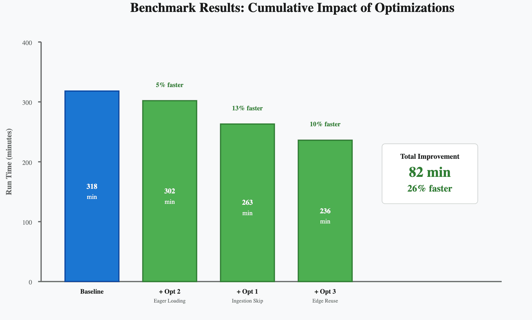
This blog discusses three new optimizations added to the Kumo platform. Across ingestion, materialization, and graph building, these optimizations reduce wasted time, often shaving 20–50% off critical stages. In production tests, these optimizations yielded 12-25% faster end-to-end training times, averaging around 20% improvement across customer workloads. These improvements are available now: version 2.11 includes initial optimizations, while 2.12 enables the full suite.

(And if you’re curious about the broader data challenges behind online training and materialization, we recommend checking out our recent post: From Toy Graphs to Billion-Node Training. It connects to similar challenges we address here.)

Understanding the Kumo Pipeline: Key Concepts

Before we dive into the optimizations, let's clarify two fundamental operations in Kumo: ingestion and graph materialization.

What Is Ingestion?

Ingestion at Kumo copies data from your source (like Snowflake, Databricks, or S3) into Kumo's secure data plane to create a stable snapshot of your data that won't change during model training and to simplify downstream operations by keeping data in a consistent, accessible location.

During ingestion, your data undergoes transformations:

• Data type conversion: You specify a data type for each column (e.g., integer, string, categorical), and Kumo converts the raw data to match these types.
• Data cleaning: Rows where the primary key or time column (timestamps indicating when data was created) contains null values are automatically filtered out.

In an iterative workflow where you're experimenting with different data types, primary keys, or time columns (collectively called the table configuration), even minor changes previously triggered a full re-ingestion. Since ingestion involves moving potentially large volumes of data between your storage and Kumo's data plane, this became a significant bottleneck during rapid experimentation.

What Is Graph Materialization?

Kumo internally represents relational databases as graphs. Rows in tables become nodes, and relationships between them (foreign keys) become edges, creating a connected structure that Graph Transformers can learn from. Graph materialization is a post-ingestion step that creates this graph representation. It involves two key steps:

Table materialization: Your ingested data is transformed into a tensor format, essentially converting rows and columns into numerical arrays optimized for machine learning. During this process, each table is also assigned a contiguous index along with its primary keys and foreign keys. These will be used for join operations during edge materialization. The tensor features are stored in Kumo's remote feature store (built on PyTorch Geometric's remote backend).

Edge materialization: Relationships between tables are created by performing join operations based on foreign keys. For example, if a "Users" table connects to an "Orders" table via a user_id, Kumo joins these tables using the contiguous indices from the previous step, and the resulting row index pairs become edges in the graph. These edges are stored in Kumo's remote graph store (also using PyTorch Geometric's remote backend).

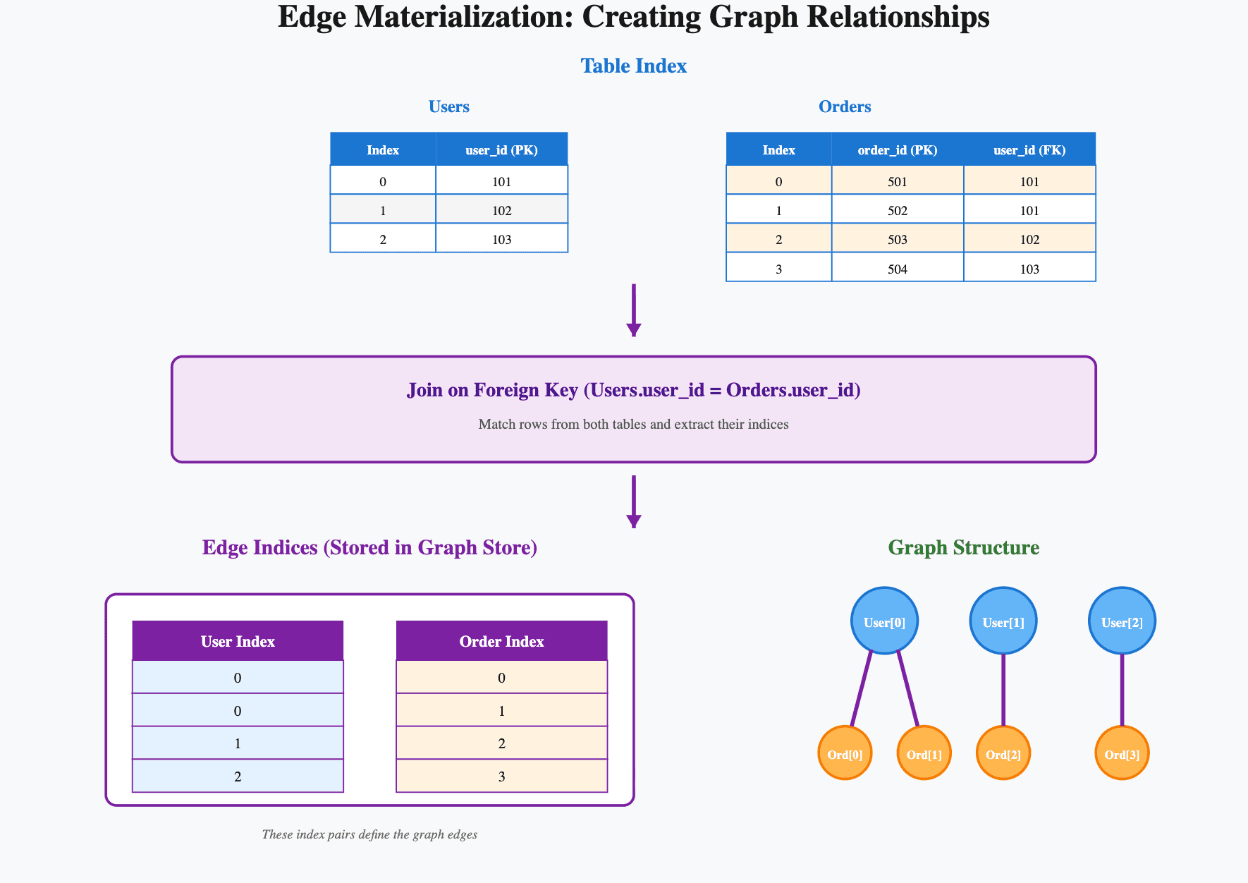
Edge materialization is particularly expensive because it requires joining potentially very large tables. As you'll see, optimizing this step was crucial to making the pipeline faster.

Optimization 1: Smarter Ingestion (Ingestion Skip)

The Issue

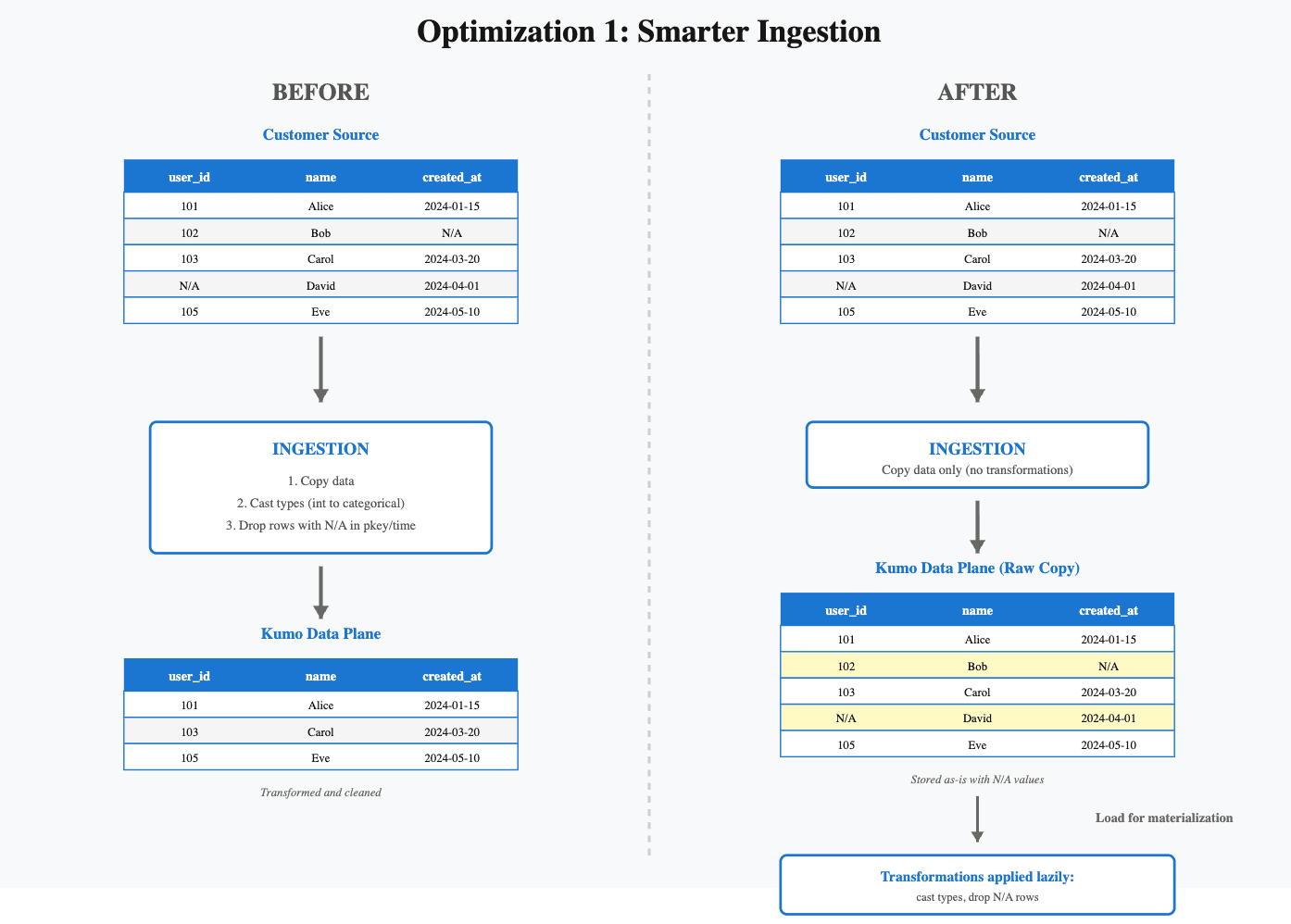
Customers frequently adjust column types or add/remove fields to experiment with how this affects model performance. The problem was that any change to your table configuration would trigger a full re-ingestion, even if the underlying source data hadn't changed.

For example, if you simply changed a column's data type from numerical to categorical or decided to use a different column as your primary key, the system would re-copy and re-transform your entire dataset. For large tables, this meant waiting through unnecessary data movement with the same data being copied again, just with slightly different transformations.

The solution

We separated table config changes from data changes. Now, ingestion is only triggered when the source data changes. Configuration changes like adjusting data types, primary keys, or time columns are made lazily when the data is needed for materialization.

To put it simply: previously, changing how you want to use your data required re-copying it. Now, we copy it once and apply your configuration preferences later in the pipeline.

The result

By decoupling config changes from ingestion, iterative schema work is dramatically faster. Refresh times are often cut by ~50% when experimenting with new graph designs.

Optimization 2: Hiding Latency with Graph Engine Eager Loading

The issue

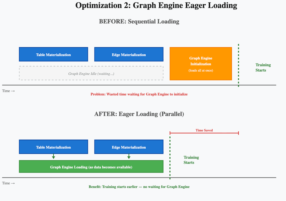
The Graph Engine, which consists of the feature store, graph store, and graph sampler, is what feeds data to the Graph Transformer during training. Previously, the Graph Engine would only start initializing after all materialization (both table and edge materialization) had completed. This created idle waiting time where no useful work was happening.

The solution

We introduced eager loading for both the feature store and graph store components of the Graph Engine. Instead of waiting for all materialization to complete before starting initialization, these components now begin loading materialized tables and edges as soon as they become available. Tables and edges are loaded into their respective stores immediately as they finish materializing. The Graph Engine is progressively warming up while other parts of the graph are still being processed.

The result

On medium-to-large graphs, customers will notice training starts 30+ minutes earlier because the wait time is compressed.

Optimization 3: Reusing Edges with Consistent Partitioning

The Issue

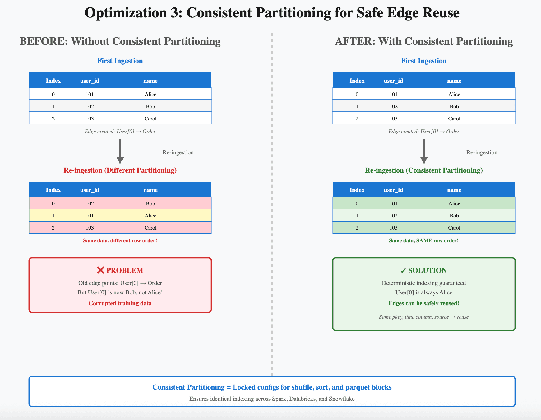
Edge materialization (building the relationships between tables) was one of the most expensive steps. Even when nothing in the underlying data changed, edges were often recomputed. Our system for detecting when cached edges could be reused (fingerprinting logic) was overly conservative.

A naive solution would be to cache and reuse edges when their table configuration looks the same. But there’s a catch: if table indexing isn’t consistent, reusing edges can silently produce row mismatches.

The solution

We built a consistent partitioning system that enforces deterministic indexing across Spark, Databricks, and Snowflake. This required careful work to ensure determinism across distributed executions to produce a contiguous table index on multiple data processing backends. The result: table indexing is now stable, so edges can be safely reused as long as the primary key, time column, and table data version remain unchanged.

Deep Dive: Why Consistent Partitioning Matters

Edge materialization involves joining tables to create graph relationships. These join operations between potentially massive tables can significantly impact runtime. At first glance, the idea of reusing edges seems straightforward. If two tables haven’t changed, why not just reuse the edge that was already materialized between them? In practice, it’s much trickier because edge materialization depends on how each table is partitioned and indexed.

When an edge is created, we take two tables and build an index that aligns rows by primary key and timestamp. If, at any point, one table gets re-ingested or rewritten with different partitioning settings (say, Spark writes with a slightly different block size, or Databricks defaults to a new shuffle config), the new table might still look identical but actually have rows ordered differently. If we naively reused the old edge, it could connect the wrong rows. That’s the kind of bug that corrupts training results silently.

To make edge reuse safe, we needed deterministic indexing across all backends: Spark, Databricks, and Snowflake. This is what we mean by consistent partitioning.

How we solved it

• Spark and Databricks: we identified the exact set of configs (shuffle partitions, sort orders, parquet block sizes) that must be locked down so that two runs produce identical index layouts.
• Snowflake: Since Snowflake doesn’t expose native indexing in the same way, we had to enforce determinism in our own implementation, especially around parquet block sizes and vectorized writes.
• Context manager: We wrapped all of this in a consistent_partitioning context manager, so that anytime a table is indexed, it is guaranteed to match prior versions if the source data is unchanged.

With this guarantee, we can now confidently reuse edges whenever the primary key, time column, and source data remain constant.

The result

This work turns edge reuse from a “maybe” optimization into a robust, default behavior. In a continuous retraining workflow, where you might be retraining daily or even hourly, this means only rematerializing a few edges that actually need updating, rather than recomputing the entire graph structure each time.

Measuring the Impact: Our Benchmarking Framework

Why we needed it

To ensure optimizations translate to real-world customer benefits, we built a benchmark suite using a synthetic version of the H&M dataset. This mirrors common usage patterns, such as running experiments with tweaks to table and graph configurations, and repeatedly training and predicting with incremental graph changes.

What it does

The framework runs these steps automatically, logs timing for each, and supports comparing optimization branches against master. Results are logged in Jenkins today, with plans to surface them in Grafana dashboards.

This ensures that version upgrades consistently bring real speedups to your workflows. In our benchmark, all three optimizations together reduced end-to-end runtime by ~25%.

Real-World Speedups in Production

While benchmarks are useful for controlled comparisons, what matters most is how these optimizations perform on real customer jobs. We tested these optimizations on real production jobs run by a well-known large food delivery company and a major social media platform.

Both customers follow the repeated training pattern: regularly retraining models as new data arrives. With the optimizations enabled, runtimes dropped significantly.

• The food delivery company saw a ~25% improvement in runtime for repeated training runs.
• At the social media platform, workloads with especially large graphs saw a 12.5% improvement. The relatively lower gain reflects that their massive scale means some operations, like model training itself, dominate runtime, while our optimizations primarily target ingestion and materialization stages

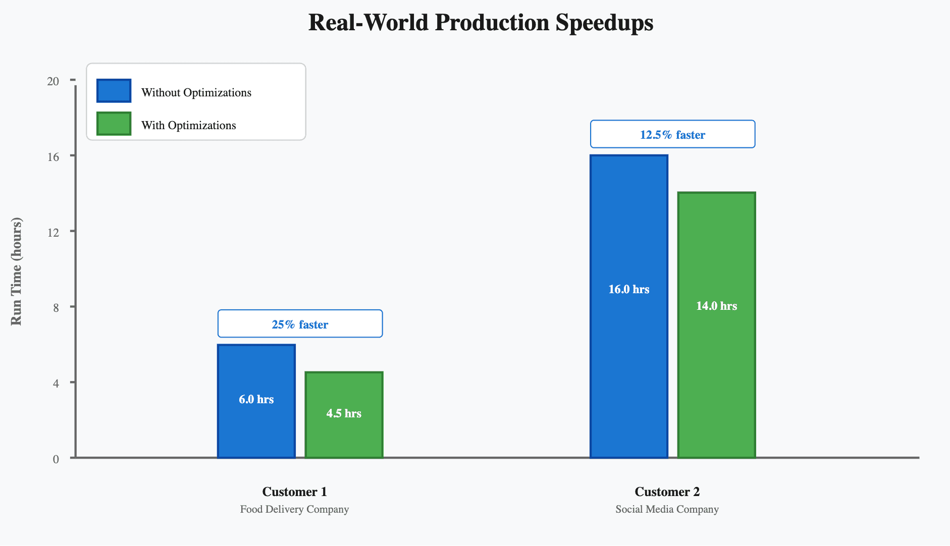
These production results reinforce the controlled benchmarks: cutting unnecessary work at the ingestion and materialization stages translates directly to faster model iteration and quicker deployment cycles.

Conclusion

By skipping unnecessary ingestion, overlapping system tasks, and reusing edges safely, we've made the Kumo pipeline faster for both iterative development and production retraining workflows.

For customers: On 2.11, you’ll already notice improvements. On 2.12, the full suite of optimizations is enabled.

Optimization is about eliminating wasted work without sacrificing correctness. These changes shorten iteration cycles so you can spend less time waiting and more time innovating.

👉 Interested in high-performance graph transformer systems? Check out our research blogs or come join us at Kumo.

Join our community on Discord.

Connect with developers and data professionals, share ideas, get support, and stay informed about product updates, events, and best practices.

Join the discussion