

If you’ve ever trained a Graph Neural Net or Graph Transformer on Cora or PubMed, you probably walked away thinking: “This isn’t so different from any other PyTorch model.” You define a couple of message-passing layers, run your training loop, and everything works.
Then you try the same thing on your company’s real data: tens of billions of nodes, dozens of edge types, terabytes of features, and edges timestamped down to the millisecond. Suddenly, your GPU isn’t the bottleneck anymore. Your jobs are stuck on data prep, your disk fills up with neighborhood dumps, and your offline metrics look suspiciously better than production.
This post is about that moment. It’s a step-by-step guide to what actually changes when you move from toy graph learning models to large-scale, production training—and how Kumo’s training backend addresses the bottlenecks that appear along the way.
1. The Hidden Complexity of Graph Learning
When you train on images, each example is a tensor of pixels. With tabular data, it’s a vector of features. These are fixed, self-contained inputs.
GNNs and Graph Transformers are different. Every example depends on a neighborhood—a dynamically constructed subgraph around the node or edge you care about. For example:
- For a recommender, the neighborhood of a user might include the items they clicked, the other users who clicked those same items, and the items those users clicked in turn.
- For fraud detection, the neighborhood of a bank account might include all the transactions it participated in, the counterparties to those transactions, and the other accounts those counterparties interacted with.
Each of these expansions adds hops, and each hop can multiply the size of the neighborhood. What starts as a single node can balloon into hundreds or thousands in just a few steps.
That’s the fundamental difference: GNNs and Graph Transformers don’t consume fixed examples, they consume constructed neighborhoods. The act of building those neighborhoods efficiently and correctly is what makes or breaks training at scale.

Caption: GNN layers aggregate information across sampled neighborhoods, much like how CNNs aggregate across receptive fields.
2. The First Attempt: Precomputing Neighborhoods with Spark
Most teams start where they’re comfortable: Spark or SQL. You can write recursive joins that traverse the graph for 2–3 hops, attach features, and write out the subgraphs as training data.
This works on small datasets. But production graphs expose its weaknesses quickly:
- Data blow-up. A single 3-hop neighborhood can be hundreds of MB. Materialize millions of them and you’ve got terabytes of intermediate data.
- Iteration is painful. Change your fanout or hop depth? Back to Spark for a full re-run.
- Neighborhoods go stale. Real graphs evolve constantly; static dumps don’t.
- Temporal leakage sneaks in. Unless you’re meticulous about time filtering, you’ll end up training on “future” edges, which inflates validation metrics but fails in production.
It’s no accident that many teams give up here: the infrastructure overhead is simply too high.
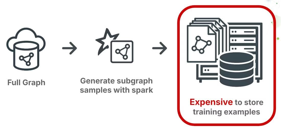
Caption: Materializing neighborhoods with Spark leads to exponential growth in storage, slow iteration, and stale training sets.
3. The Shift: Online Sampling
The way forward is to stop precomputing and start sampling neighborhoods online. Instead of treating neighborhoods as static data, you treat them as queries: each batch asks for a fresh neighborhood, sampled just in time.
This pattern emerged independently at large companies like Pinterest (PinSage) and Alibaba (AliGraph). At Kumo, we’ve built a backend that packages the same approach into something engineers and data scientists can use directly.
Here’s how it works:
- Graph Sampler (RAM): The sampler holds the graph structure in memory for ultra-fast lookups. It expands neighborhoods according to your configuration: hop depth, fanouts per edge type, metapaths, and time constraints. Temporal correctness is enforced automatically—you only ever see edges valid at the time of the training example.
- Feature Store (SSD): The sampler returns node IDs. The feature store fetches their attributes from SSD storage. This allows you to work with terabytes of features without overloading GPU memory.
- GPU Trainer (PyTorch): Once you have the subgraph and its features, the rest looks familiar. You run it through your GNN or transformer layers, compute a loss, and backpropagate.
The entire pipeline is built to generate thousands of neighborhoods per second, keeping GPUs saturated without filling up disks.
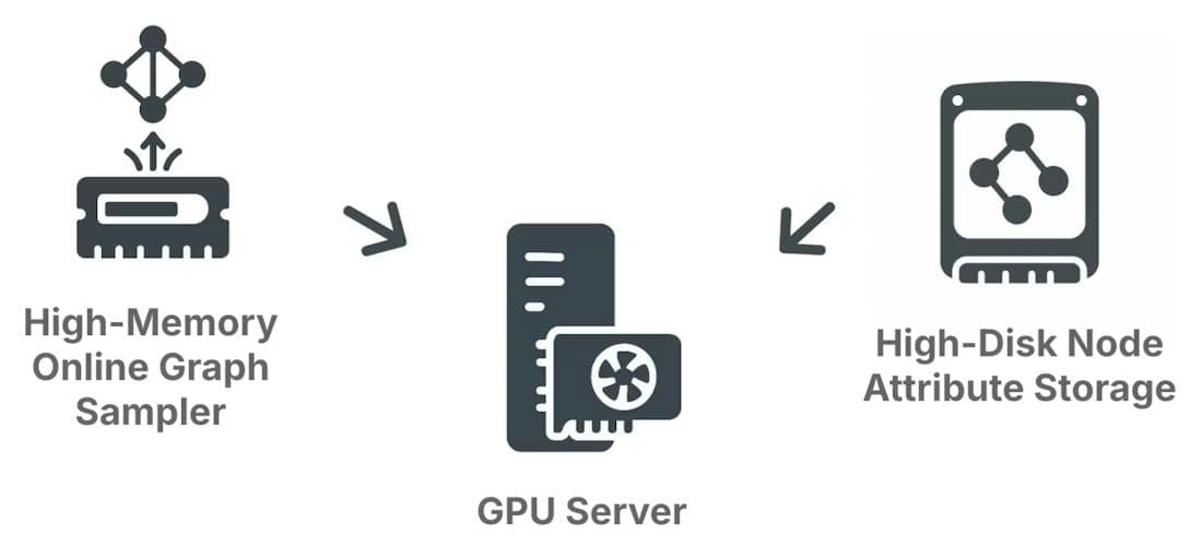
Caption: Online neighborhood sampling: the sampler, feature store, and GPU trainer work together to build neighborhoods just in time.
4. What This Architecture Enables
By shifting to online sampling, you unlock scale that was previously infeasible. For example:
| Parameter | Example Capability |
|---|---|
| Graph Size | 10–30 Billion nodes (1TB server) |
| Subgraph | 6+ hops (on sparse graphs) |
| Depth Inference | Batch or Online (inductive) |
| Sampling | Static or Temporal (per metapath) |
Instead of being limited to shallow 2-hop neighborhoods, you can train deeper models that aggregate context over 6+ hops. Instead of offline metrics collapsing in production, you can enforce temporal correctness at sampling time. And instead of being stuck with static dumps, you can run batch inference or score brand-new nodes online using the same pipeline.
5. Relating Back to PyTorch
If you’re already comfortable with PyTorch, the analogy is straightforward.
- The graph sampler is like a DataLoader. Instead of rows, it emits subgraphs.
- The feature store is like a collate_fn, attaching attributes to nodes and edges in the batch.
- The model is still an nn.Module. Whether you use GraphSAGE, GAT, or a transformer, it plugs in here.
Your training loop doesn’t change much. You still fetch batches, run them through the model, compute a loss, and optimize. The only difference is that each “batch” is now a freshly constructed neighborhood.
6. Working with Real Graphs
Toy benchmarks usually show simple, homogeneous graphs. Real production graphs look very different: multiple node types, multiple edge types, and timestamped interactions. Training at scale means controlling how neighborhoods are sampled, not just how many layers your model has.
In Kumo, this is exposed through the num_neighbors parameter. This setting tells the sampler how many neighbors to expand at each hop. For example, you might configure:
1num_neighbors:
2- hop1:
3    default: 16
4- hop2:
5    default: 8
This means: sample up to 16 neighbors per connection at the first hop, and up to 8 at the second hop. By chaining hops together, you can go as deep as 6 hops on sparse graphs.
You can also override these defaults on a per-edge basis. Suppose you want to emphasize user-to-transaction links but ignore certain transaction-to-store edges. You can write:
1num_neighbors:
2- hop1:
3    default: 16
4    USERS.USER_ID->TRANSACTIONS.USER_ID: 128
5- hop2:
6    default: 8
7    TRANSACTIONS.STORE_ID->STORES.STORE_ID: 0
Here, the sampler pulls up to 128 transactions per user in the first hop, but skips store sampling entirely in the second hop. This kind of fine-grained control is crucial in messy, heterogeneous domains like fraud or recommendation, where not all relationships are equally important.
Temporal strategies are supported too. By default, Kumo weights newer edges more heavily, but you can flip to uniform sampling if that’s what your task requires. For certain connections, you can even let Kumo infer the best fanout based on degree statistics.
The bottom line: real-world GNNs and Graph Transformers aren’t just about stacking layers. They’re about shaping neighborhoods to match your problem domain—and parameters like num_neighbors give you the knobs you need.
7. Putting It Into Practice
Here’s what working with Kumo looks like end to end:
- Define your task. Use a Predictive Query to specify the entity you’re predicting for (e.g. user churn, fraud risk).
- Generate a ModelPlan. The SDK can suggest one (pquery.suggest_model_plan()), which you can then customize. See the SDK trainer reference.
- Configure sampling. Neighborhood expansion is controlled through num_neighbors, with per-hop and per-edge fanouts.
- Train your model. Launch training with the Trainer API. Batches are generated online, so GPUs always see fresh neighborhoods.
- Run inference. Use the same sampler settings for batch prediction or online scoring, ensuring consistency between training and serving.
From your perspective as an engineer or data scientist, it feels like working with PyTorch and a smarter data loader. The heavy lifting—fast sampling, feature streaming, time correctness—happens under the hood.
8. Takeaways
Graph learning at scale teaches a simple lesson: the bottleneck isn’t the math, it’s the neighborhoods.
- Precomputing with Spark doesn’t scale.
- Online sampling is the architecture that works in practice.
- With the right backend, billion-node graphs are trainable, and graph learning feels approachable again.
So the next time you see a new graph learning paper and wonder, “But will this run on our data?” — the answer is yes, as long as your neighborhood pipeline can keep up.
Join our community on Discord.
Connect with developers and data professionals, share ideas, get support, and stay informed about product updates, events, and best practices.