
A quiet paradigm shift is underway in machine learning. For most of the last decade, progress came from building bigger or more efficient models: gradient-boosted trees, deep neural networks, and transformer architectures for language and vision. The focus was on scale and speed.
Now, the shift is conceptual. Instead of seeing data as rows in a table, models are beginning to learn directly from relationships — the way entities interact, influence, and depend on each other over time. This change is redefining predictive modeling itself.
Graph Neural Networks (GNNs) and, more recently, Graph Transformers, are leading this shift. They make it possible to capture relational and temporal structure in complex datasets, from supply chains and energy grids to molecules and experiments.
Kumo’s platform operationalizes this idea, bringing these research-grade architectures into the hands of data scientists in a form that fits naturally alongside Python’s open-source ecosystem.
From Tables to Networks
Traditional predictive workflows assume that data points are independent. Customers, transactions, products, or time steps all treated as separate rows. That assumption simplifies modeling, but it erases the connected nature of real systems.
In practice, few datasets are truly independent.
- Demand for one product often depends on related products, suppliers, and promotions.
- Sensor readings are correlated across networks of equipment.
- Molecular interactions depend on shared structural or biochemical properties.
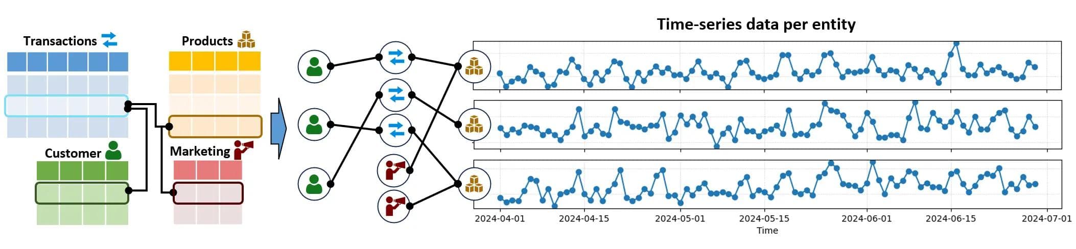
Graph-based learning changes this representation. Each entity becomes a node, each relationship an edge. The model learns not only from what each node looks like, but from how it connects to others. Context becomes part of the data.
Image: Relational tables forming a graph and time-series per node
Forecasting with Structure
Forecasting is one of the clearest examples of how this shift plays out.
Classic approaches (ARIMA, Prophet, LightGBM) are designed to forecast each time series independently. That’s fine for isolated signals, but in many systems, time series are coupled.
Sales of related SKUs rise and fall together. A delay in one supplier can ripple downstream through an entire logistics network. Temperature sensors on connected equipment display shared patterns of drift.
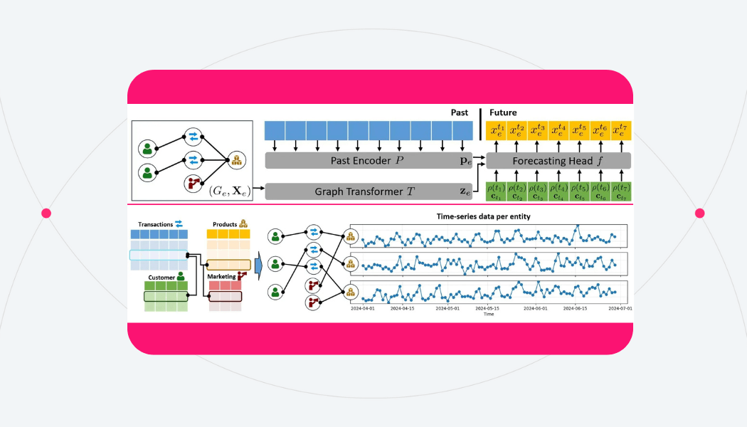
Graph Transformers treat these correlations as part of the model itself. Each entity has a time series and connections to other entities. The model learns from both, using temporal encoders to capture local history and graph encoders to share information across related entities.
Image: Graph + past-sequence encoder architecture
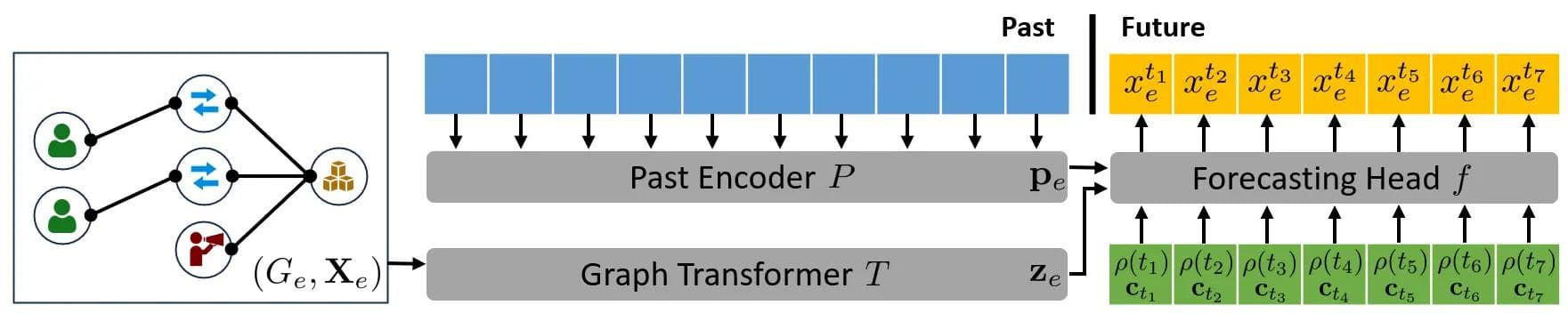
This combination allows for richer, context-aware forecasts - models that understand how systems move together, not just how individual signals evolve in isolation.
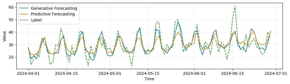
Image: Forecast comparison Generative Graph Transformer outputs retain high-frequency detail compared with Prophet and baseline models. To learn more, check out the full blog post here.
Why Graph Transformers Work So Well
Graph Neural Networks already made it possible to model structured relationships, but their reach is often limited to local neighborhoods. As graphs grow deeper, signals tend to blur, a challenge known as over-smoothing.
Graph Transformers solve this through attention-based mixing, allowing information to travel across distant nodes while maintaining local specificity.
Image: GNN message passing vs. global attention
The result is an architecture that can model both fine-grained and system-wide dynamics in a single framework, effectively combining the reasoning strength of graphs with the representational power of transformers.
A Declarative Way to Work
Building these models from scratch used to take thousands of lines of code: managing joins, temporal windows, leakage control, negative sampling, and MLOps. The Kumo SDK replaces that boilerplate with a few simple, declarative steps.
Here’s an example drawn from a real biotech workflow: predicting protein–ligand interactions using a knowledge graph of five connected tables.
1import kumoai as kumo
2
3# Initialize the Kumo SDK
4kumo.init(...)
5connector = kumo.SnowflakeConnector(...)
6
7# Create Kumo tables
8proteins = kumo.Table.from_source_table(
9    source_table=connector.table("PROTEINS"),
10    primary_key="PROTEIN_ID"
11).infer_metadata()
12
13ligands = kumo.Table.from_source_table(
14    source_table=connector.table("LIGANDS"),
15    primary_key="LIGAND_ID"
16).infer_metadata()
17
18interactions = kumo.Table.from_source_table(
19    source_table=connector.table("PROTEIN_LIGAND_INTERACTIONS"),
20    primary_key="BIOACTIVITY_ID"
21).infer_metadata()
22
23protein_interactions = kumo.Table.from_source_table(
24    source_table=connector.table("PROTEIN_PROTEIN_INTERACTIONS"),
25    primary_key="PPI_ID"
26).infer_metadata()
27
28ligand_similarities = kumo.Table.from_source_table(
29    source_table=connector.table("LIGAND_LIGAND_SIMILARITIES"),
30).infer_metadata()
31
32# Create a graph connecting the tables
33bioactivity_graph = kumo.Graph(
34    tables={
35        "proteins": proteins,
36        "ligands": ligands,
37        "interactions": interactions,
38        "protein_interactions": protein_interactions,
39        "ligand_similarities": ligand_similarities
40    },
41    edges=[
42        dict(src_table="interactions", fkey="PROTEIN_ID", dst_table="proteins"),
43        dict(src_table="interactions", fkey="LIGAND_ID", dst_table="ligands"),
44        dict(src_table="protein_interactions", fkey="PROTEIN1_ID", dst_table="proteins"),
45        dict(src_table="ligand_similarities", fkey="LIGAND1_ID", dst_table="ligands"),
46        dict(src_table="ligand_similarities", fkey="LIGAND2_ID", dst_table="ligands")
47    ]
48)
49
50link_prediction_pquery = kumo.PredictiveQuery(
51    graph=bioactivity_graph,
52    query=(
53        "PREDICT LIST_DISTINCT(interactions.LIGAND_ID)\n"
54        "RANK TOP 10\n"
55        "FOR EACH proteins.PROTEIN_ID\n"
56    )
57)
58
59# Train the link prediction model
60link_trainer = kumo.Trainer(link_prediction_pquery.suggest_model_plan())
61link_training_job = link_trainer.fit(
62    graph=bioactivity_graph,
63    train_table=
64link_prediction_pquery.generate_training_table(non_blocking=True)
65)
66
That’s the full pipeline in about 60 lines: data connection, feature generation, model selection, training. The same task in CatBoost or even PyTorch would require thousands: joining/aggregating data into a single flat training table (dropping information in the process), and then engineering complex features in order to coax the model in to picking up the signal that was lost.
The graph transformer automatically learns features that would otherwise be hand-crafted:
- Protein–protein and ligand–ligand relationships through multi-hop connections.
- Similarity-based effects that emerge from shared molecular structure.
- Temporal patterns that evolve across experiments without manual windowing.
The result is not just fewer lines of code, but a clearer way to express what the model should learn.
To learn more, you can check out the documentation for the Kumo platform as well as Kumo’s python SDK.
Control Where It Matters: Advanced Options for Power Users
While Kumo handles much of the engineering overhead, it’s not a black box. The best results still depend on domain expertise, particularly in how the relational graph is constructed and how the model explores it.
Data scientists and subject-matter experts define the network of learning: which entities are included, which relationships connect them, and how far information should travel. This design shapes what the model can see and what it can infer.
Kumo’s Model Planner exposes the same level of configurability found in open-source frameworks like PyTorch Geometric (github.com/pyg-team/pytorch_geometric), which Kumo’s researchers helped author. Every layer, aggregation, and sampling step can be adjusted with defaults that align to proven research practices.
For example, controlling neighborhood sampling through the num_neighbors parameter defines how many connected nodes each entity attends to during training. Increasing it broadens context, allowing the model to capture long-range dependencies; constraining it enforces locality and reduces noise.
1model_plan = pquery.suggest_model_plan()
2
3model_plan.override(
4    neighbor_sampling=dict(
5        num_neighbors=[
6            {"hop": 1, "default": 10},
7            {"hop": 2, "default": 5},
8            {"hop": 3, "default": 2},
9        ]
10    ),
11    model_architecture=dict(
12        graph_transformer=dict(
13            channels=[256],
14            num_heads=[8],
15            num_layers=[3],
16        )
17    ),
18)
19
Neighborhood size, message-passing depth, and attention heads together control the effective “field of view” for each node, a powerful lever for domain experts who know which connections carry real signal.
Other options include:
- Edge-type weighting, letting certain relationships (e.g., ligand–ligand vs. assay–ligand) carry more influence.
- Custom aggregation functions, such as mean, sum, or attention-based pooling.
- Feature selection and masking, useful when some columns represent experimental noise.
- Embedding sharing and reuse across tasks, allowing one trained graph to seed another.
This interface is what makes declarative relational modeling practical. It removes repetitive work without removing the role of expertise.
Looking Ahead
Graph Transformers represent more than another incremental model improvement. They reflect a broader rethinking of how predictive systems understand the world, as networks of influence rather than lists of records. In short, machine learning is starting to model the world as it actually is: connected.
Join our community on Discord.
Connect with developers and data professionals, share ideas, get support, and stay informed about product updates, events, and best practices.